Normalizable wave function
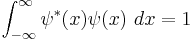
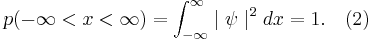
In quantum mechanics, wave functions which describe real particles must be normalizable: the probability of the particle to occupy any place must equal 1. [1] Mathematically, in one dimension this is expressed as:
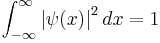
Or identically:
where the integration from  to
to  indicates that the probability that the particle exists somewhere is unity.
All wave functions which represent real particles must be normalizable, that is, they must have a total probability of one - they must describe the probability of the particle existing as 100%. For certain boundary conditions, this trait enables anyone who solves the Schrödinger equation to discard solutions which do not have a finite integral at a given interval. For example, this disqualifies periodic functions as wave function solutions for infinite intervals, while those functions can be solutions for finite intervals.
Contents |
Derivation of normalization
In general,  is a complex function. However,
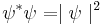
is real, greater than or equal to zero, and is known as a probability density function. Here,  indicates the complex conjugate.
This means that
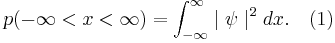
where  is the probability of finding the particle at
  . Equation (1) is given by the definition of a probability density function. Since the particle exists, its probability of being anywhere in space must be equal to 1. Therefore we integrate over all space:
If the integral is finite, we can multiply the wave function, , by a constant such that the integral is equal to 1. Alternatively, if the wave function already contains an appropriate arbitrary constant, we can solve equation (2) to find the value of this constant which normalizes the wave function.
Plane-waves
Plane waves are normalized in a box or to a Dirac delta in the continuum approach.
Example of normalization
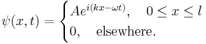
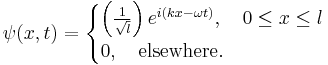
A particle is restricted to a 1D region between  and
and  ; its wave function is:
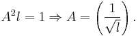
To normalize the wave function we need to find the value of the arbitrary constant  ; i.e., solve
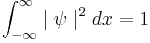
to find .
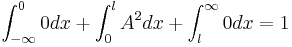
Substituting into  we get

so,
therefore;
Hence, the normalized wave function is:
Proof that wave function normalization does not change associated properties
If normalization of a wave function changed the properties associated with the wave function, the process becomes pointless as we still cannot yield any information about the properties of the particle associated with the un-normalized wave function. It is therefore important to establish that the properties associated with the wave function are not altered by normalization.
All properties of the particle such as: probability distribution, momentum, energy, expectation value of position etc.; are derived from the Schrödinger wave equation. The properties are therefore unchanged if the Schrödinger wave equation is invariant under normalization.
The Schrödinger wave equation is:
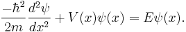
If is normalized and replaced with  , then
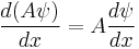 and
and 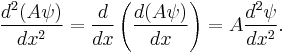
The Schrödinger wave equation therefore becomes:
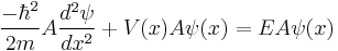
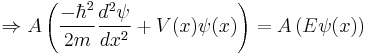
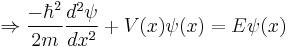
which is the original Schrödinger wave equation. That is to say, the Schrödinger wave equation is invariant under normalization, and consequently associated properties are unchanged.
See also
References
- ^ Griffiths, David J. (April 10, 2004). Introduction to Quantum Mechanics. Benjamin Cummings. p. 11. ISBN 0131118927.
External links
- [1] Normalization.